|
||||||||||||||||||||||||||||||
|
This task is
focused on the normalization of the facial surface based on a reduced set of manual
annotations and has been addressed by implementing Least Squares Conformal
Maps (LSCM). The conformality condition ensures that the angles (of the mesh
triangles used to describe the facial surface) are locally preserved, hence
minimizing mapping distortion. Applying LSCM
to synthetic or carefully pre-processed data is rather straight-forward.
However, when using real-World data (e.g. generated by scanning human faces)
there is some probability in obtaining an underdetermined system of
equations. In the specific case of our input data, this problem affected
about 20% of the input surfaces. In a subset of these, the underdetermination led to artifacts in the generated
mapping. The main causes for underdetermination
were the presence of singularities and disconnected regions in the surface.
From a theoretical point of view this is reasonable because the relations
between neighbouring triangles can only be computed
if there is a common edge, which is not available at the aforementioned
cases. Removing these
artifacts resulted in well-determined systems, thus allowing the correct
computation of the conformal mapping. Once this is achieved, it is possible
to compute a dense correspondence between all input surfaces. Indeed, we can
also re-sample them by inverting the conformal mapping. This has the
advantage of providing a new representation of the input surfaces with
corresponding vertices for all of them, allowing their analysis with standard
multivariate methods. |
||||||||||||||||||||||||||||||
|
Least Squares Conformal Mapping |
||||||||||||||||||||||||||||||
|
Given that the
face is (approximately) a genus-0 surface, it can be mapped conformaly into the 2D domain. The conformality
condition ensures that the angles are locally preserved, hence minimizing
mapping distortion. Under such constraints, there is a family of possible
solutions with 6 degrees of freedom, related by the group of Möbius transformations [Li
2006]. At least two corresponding points are needed to make the
solution unique, but additional points can be added in order to obtain a
least squares solution, which would balance the localization errors of
individual points [Wang 2007]. This
technique was introduced by Levy et al. [Levy 2002]
as Least Squares Conformal Mapping (LSCM). Given a
surface S in terms of its 3D coordinates {x,y,z} we can define a 2D parameterization {u, v} Ì R2 so that the surface is locally
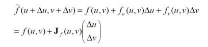
defined by the mapping f(u,v) ® {x,y,z}. The 1st
order Taylor approximation of f(u,v) with
infinitesimal displacements Du, Dv is:
where fu
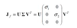
and fv are partial derivatives and Jf(u,v) is that Jacobian matrix,
which can be decomposed as follows:
We are
interested in the eigenvalues of S, i.e. s1 and s2. These
are important to determine the type of metric distortion introduced by the
mapping f, as follows: ·
f is
isometric or length-preserving « s1 = s2 = 1 ·
f is
conformal or angle-preserving « s1 = s2 ·
f is equiareal or area-preserving « s1 s2 = 1 Because the
equality of the eigenvalues of J implies equality for those of J-1, the inverse mapping (i.e. the one from 3D to 2D)
is also conformal. It shall be noted that LSCM produces a mapping that is
approximately conformal, as it is well known that a discrete surface cannot,
in general, be mapped into 2D under strict conformality.
In [Hormann 2007] a practical implementation of LSCM is
derived by noting that for a mapping to be conformal we need the gradients
with respect to the parameterization variables to be orthogonal and have the
same norm:
where rot90 is a 90 degree rotation
(anti-clockwise in this case) and the gradients of u and v are taken with
respect to a local coordinate system placed at each triangle of the surface.
Thus, we end up with 2 equations per triangle that are linear in the vertex
coordinates (in terms of u and v). The resulting system of equations will be
underdetermined unless we fix the coordinates of 2 or more points. Once this
is done the system is well-determined (as long as there are no surface artifacts like those mentioned in Section 2.1). A typical
facial scan from the datasets analyzed in this project contain between 50,000
and 300,000 triangles. With two equations per triangle, it is evident that
the size of the resulting system is considerable. Fortunately, the system is
also very sparse and can therefore be satisfactorily handled with libraries
such as UMFPACK.
|
||||||||||||||||||||||||||||||
|
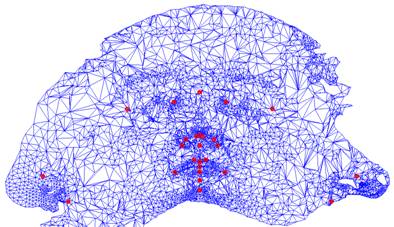
An interesting
aspect of the mapping illustrated in Fig. 1 is that the coordinates of the landmarks
that are used as correspondences between 2D and 3D vary only in 3D but can be
maintained fixed in 2D. That is, given a set of surfaces in 3D with the same
set of anatomical landmarks annotated, they can be mapped into 2D so that
those landmarks are coincident. This implies that, except for the distortion
introduced by the conformal mapping, we have a common reference frame where a
given 2D coordinate has the same anatomical meaning for all meshes that have
been mapped. The above, however,
has an important practical limitation: the mapping is a piecewise linear
function, which is defined for each mesh only at the vertices of its
triangulation. In the general case different surfaces have different
triangulations and their vertices will be mapped into non-coinciding
coordinates in the 2D domain. Hence, if we
want to generate a representation that is homologous across surfaces we need
to re-sample them. For this purpose we adopted a two-step approach:
While the
above procedure can be applied individually to each surface, such a strategy
would again result in different sampling positions of the 2D domain. It is
preferable, instead, to apply the same sampling grid to the whole population
of surfaces that have to be analyzed, so that these points can be considered
pseudo-landmarks. Once this is done, all surfaces have a homologous
representation and we can apply standard multivariate analysis techniques. |
||||||||||||||||||||||||||||||
|
References |
||||||||||||||||||||||||||||||
|
[Alliez 2003] P. Alliez, E.C. Verdiere,
O. Devillers et al. Isotropic
Surface Remeshing. Proc. Int. Conf. Shape Modeling, pp.
49-48, 2003. [Hormann 2007] K. Hormann, B. Levy
and A. Sheffer. Mesh
Parameterization: Theory and Practice. ACM SIGGRAPH course notes,
2007. [Levy 2002] B. Levy, S. Petitjean
and N. Ray et al. Least
Squares Conformal Maps for Automatic Texture Atlas Generation. Proc.
Int. Conf. Computer graphics and interactive techniques (SIGGRAPH), pp.
362-371, 2002. [Li 2006] H. Li and R. Hartley. New 3D Fourier
descriptors for genus-zero mesh objects. In Proc. Asian Conference on
Computer Vision. LNCS vol. 3851, pp 734–743, 2006. [Wang 2007] S. Wang, Y. Wang, M. Jin et al. Conformal
Geometry and Its Applications on 3D Shape Matching, Recognition, and
Stitching. IEEE Transactions on Pattern Analysis and Machine Intelligence,
29(7):1–12, 2007. |
||||||||||||||||||||||||||||||
|
|
||||||||||||||||||||||||||||||
|
|
|
|
|
|||||||||||||||||||||||||||