|
||||||||||||||||||||||||||||||
|
This task is
focused on the implementation of state-of-the-art algorithms for Spectral
Mesh Processing (SMP) for their application to the analysis of craniofacial
geometry. SMP is a novel branch of computer geometry and vision that focuses
on the analysis of surfaces embedded in 3D based on the decomposition of the
geometry in the frequency domain [Zhang 2010]. Analogous to the Fourier decomposition employed
in signal processing, the seminal work by Taubin [Taubin 1995] suggested
that the spatial frequencies of a 3D surface (described as a triangulated
mesh) could be computed from the eigendecomposition
of the Laplacian operator. The wide
interest attracted by SMP soon revealed an important shortcoming. In its
original formulation, Taubin shows that the Fourier
decomposition of a 1D signal arises from the eigendecomposition
of the Laplacian (also in 1D) and extrapolates this result to 3D using the so
called combinatorial graph Laplacian. This combinatorial operator perfectly
emulates its 1D counterpart, but it is based only on the connectivity of the
mesh, without taking into account its geometric information. While this is
acceptable in 1D, where the signals are sampled at equidistant intervals
(i.e. uniform sampling), it does not suffice for surfaces embedded in 3D. In
the latter, the geometry is usually represented by triangulations (simplicial complexes) which are almost invariably
non-uniform regarding their size and their angles.
More
rigorously, the Laplacian can be considered a special case of the more
general Laplace-Beltrami Operator (LBO), which is defined on a manifold
invariant to its parameterization, taking into account only its Riemannian
metric [Reuter 2006, Bronstein 2011]. The most widely accepted formulation for the LBO
on 3D meshes is based on the cotangent weights [Meyer 2002], derived
from the continuous definitions of the surface curvature assuming that the
geometry is reasonably approximated by the triangulation at hand. Further
research has addressed the problem from different perspectives, mainly by
employing Finite Elements or Discrete Exterior Calculus (DEC). The results
are still based on the cotangent weights but it has been shown that a
correction factor is needed for the operator to fulfil
the mathematical properties of the (continuous) LBO [Levi 2006, Vallet 2008]. Another way
to intuitively understand LBO eigenfunctions is to
think of them as the generalization of spherical harmonics [Li 2006, Khairy 2008] to other
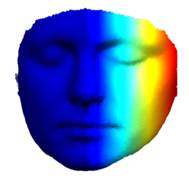
non-spherical geometries. Fig. 1 shows examples of some eigenfunctions
of the LBO in a facial surface. The spectrum
of the LBO is an isometric invariant, and it has been shown to be a powerful
descriptor as a signature for 3D shape matching and classification [Reuter 2006, Ruggeri 2010]. Among several
properties, its nodal sets (the zero-sets of its eigenfunctions)
are known to divide the surface in (at most) as many regions as the order of
the eigenfunction, defining curves that intersect
at constant angles [Levy 2006]. Thus, they are strongly linked to the geometry of
the surface and its intrinsic structure [Qiu 2008]. It has been observed that level sets of LBO eigenfunctions follow geometric features [Levy 2006], highlight
protrusions [Reuter 2010] and reveal (global) symmetry, which is considered
very important in dysmorphology [Hammond 2008, Qiu 2009, Atmosukarto 2010]. |
||||||||||||||||||||||||||||||
|
Discrete operators using cotangent weights |
||||||||||||||||||||||||||||||
|
The Given a surface S (2-mainold) embedded in R3,
we can locally approximate it at any point by its tangent plane, orthogonal
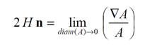
to the normal vector n. Given the
mean curvature H and an infinitesimal area element A with diameter diam(A), the following holds:
where Ñ is the gradient with respect to the 3D coordinates
(at the point being considered). Meyer et al. define their LBO as L = 2 H n. The above
equations regard to the continuous setting. To extend them to the discrete
setting, each vertex is considered in a neighbourhood AM, which is
restricted to be within its 1-ring neighbourhood, where spatial averaging is
performed. The exact calculation of AM depends on whether the
triangles in the 1-ring are obtuse or not but, conceptually, it is an
approximation of the Voronoi region of the
considered vertex appropriately corrected to deal with bad conditioned cases.
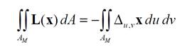
The LBO of the
surface with respect to the conformal space parameters u and v, conveniently
chosen as the current surface discretization (i.e. using directly the surface
triangles) becomes simply the flat space Laplacian Du,v. Then:
From this
point, spatial averaging is derived from finite element techniques, using a
linear finite element on each triangle (i.e. to interpolate between the
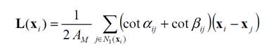
vertices). Using Gauss’s theorem with appropriate algebraic manipulation [Meyer 2002] leads to:
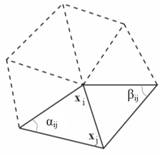
where N1(xi)
is the set of 1-ring neighbours of xi, and the angles αij and βij
are always those opposite to the edge formed by xi and xj,
as in the example of Fig. 2. Applying the same strategy, discrete operators
for the normal vector, mean curvature and Gaussian curvature are also derived
(and have been implemented).
|
||||||||||||||||||||||||||||||
|
Discrete
operators using the heat kernel |
||||||||||||||||||||||||||||||
|
In contrast to
the operators described in the previous section, we also implemented an
alternative approach to compute the LBO presented by Belkin
et al. [Belkin 2008]. It is also
based on an approximation of integrals on a discretized
surface but the authors combine it with the idea of approximating the heat
flow on a mesh. The most attractive feature of the algorithm is that it
guarantees point-wise convergence of the derived approximation to the correct
LBO. Let M={X,
T} be a triangulated mesh, obtained by sampling a surface S, composed by
two sets: the vertices X = {x}
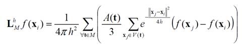
and the triangles T = {t}. Given a function f : X ® R, Belkin’s algorithm approximates the LBO of the function
at vertex xi as:
where h is a
parameter that controls the size of the diffusion kernel, A(t) is the area of
a given triangle and V(t) is the set of its vertices. Note that the
neighborhood considered for vertex xi depends on h and is not limited to the
1-ring neighborhood. Thus, it might seem that the connectivity of the mesh
does not play a role in the above equation, but it does in two different
ways: 1.
The
distances between vertices, used in the exponential, should in reality be
computed as Geodesics. The use of Euclidean distances is only an
approximation intended for small enough neighborhoods. 2.
For each
triangle we end up with a common coefficient (or weight) that is split evenly
among its vertices. Thus, the resulting weight for a given vertex depends on
its valence (the number of triangles in its 1-ring neighborhood). Apart from
providing a guaranteed convergence, this approach is more flexible than the
one by Meyer et al. because it allows controlling the size of the
neighborhood that is considered with the diffusion parameter. However, when
assessing the correctness of the operator for some synthetic cases, we found
that convergence is achieved only for extremely fine tessellations and
neighborhoods that are considerably larger than the 1-ring of the considered
vertex. Apart from the
derivations from cotagent weights (including a few
variants with the same core algorithm) and diffusion kernel, there are also
interesting alternatives based on finite element approximations of higher
order that bypass the computation of the LBO and address directly the
generation of its spectrum [Reuter 2009], which is indeed our ultimate goal. |
||||||||||||||||||||||||||||||
|
Comparison of discrete Laplacian operators |
||||||||||||||||||||||||||||||
|
Different
algorithms to compute the Laplacian operator are typically compared by
applying them to some simple function in domains such as planes or spheres.
The reason for restricting the evaluation to such simple cases is the
possibility to compute the correct Laplacian analytically. Actually, an
interesting aspect of the evaluation is that we cannot directly evaluate the
correctness of the operator; instead, we need to apply to operator to a
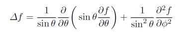
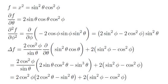
function and evaluate the result. For the tests
reported below we used a non-linear function f defined on the sphere, f : S2
® R = x2, as done by Belkin
et al. [Belkin 2008]. Because the
function is defined only in the unit sphere, the analytic solution for the
Laplacian of f is:
where θ and ϕ are, respectively, the elevation azimuth angles in
spherical coordinates. Recall that we are under the simplification of a unit
sphere, hence that radius is 1 and we omit it everywhere. Thus, x =
sin θ cos ϕ and we
get:
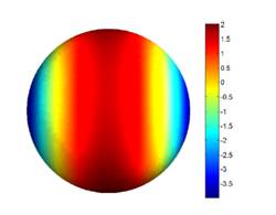
Fig. 3 shows
the analytic result, color-coded into the surface of the sphere.
To evaluate
the quality of the operators, we used 3 different discretizations
of the sphere: the first one was generated by a uniform sampling in the
azimuth-elevation plane, which implies a higher sampling density near the
poles, and the other two were generated with near-uniform sampling in the
spherical domain. However, the latter two were differed in the approximation
used to generate the uniform sampling: therefore, they had some differences
in the underlying triangulation. In all three cases, the spheres had
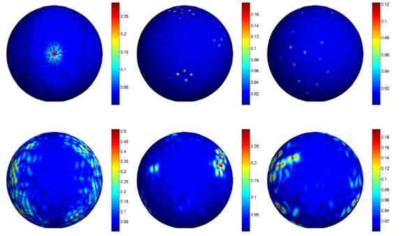
approximately 8000 points. Visually, both operators look very similar to the
analytic result displayed in Fig. 3 on all three discretizations.
However, if we plot the absolute difference between the discrete operators
and the analytic result we can clearly appreciate some differences, as shown
in Fig. 4.
The main
conclusion we can extract is that the operator based on cotangent weights [Meyer 2002] is more accurate
and, especially, more consistent. The latter is clear when comparing the two
spheres with near-uniform sampling, where the operator based on heat
diffusion creates error patterns that are quite different between these two
cases. It is also interesting to note that, in the non-uniform case, the
cotangent-based operator has bigger errors in the poles, where the sampling
density increases and the triangles become more elongated. On the other hand,
the method based on heat diffusion does not have problems in the poles,
because the higher sampling density helps to achieve a better approximation
to the integral. |
||||||||||||||||||||||||||||||
|
Quantitative comparisons on spheres of variable
density |
||||||||||||||||||||||||||||||
|
Our results reported
above confirm the statements from the related literature, which indicate that
the operator based on cotangent weights produces more accurate and consistent
results than the heat diffusion operator but only for idealized cases as it
could be more affected by noise and uneven triangulations. Indeed, both
approaches have some problems related to the triangulation. The cotangent
operator has problems for triangles with large difference in edge sizes (i.e.
with big aspect ratios) and the heat diffusion operator is sensitive to the
valence of vertices (the number of adjacent triangles). In the case of the
heat diffusion operator, however, this problem is partially tackled by the
fact that a relatively large neighborhood is considered for each point; integration
over the neighborhood tends to compensate the small deviations introduced
individually by each point but that also increases the size of the
neighborhood that we need to take. Larger neighborhoods are undesirable for
several reasons: they take longer to process, require move memory and reduce
the locality of the operator, which might therefore not be able to capture
enough detail. An interesting
aspect of the diffusion operator is that its dependency with the valence of the
vertices could be easily removed, or at least attenuated. The reason for this
dependency is that the contribution of each vertex is weighted by a factor
proportional to the area of the incident triangles: actually, each vertex of
a triangle gets exactly one third of the area-weight of that triangle. This
is of course suboptimal and a very reasonable approximation has been provided
by Meyer et al. [Meyer 2002] to construct a Voronoi
tessellation of the mesh. Hence, apart from the two original methods (cotangent
and heat diffusion), we tested a third one (diffusion + Voronoi)
which is the (rather trivial) extension of the heat diffusion method with the
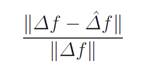
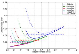
Voronoi areas from the cotangent-based method. Fig. 5 shows
the normalized L2 error on uniformly sampled spheres of variable
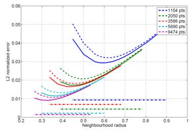
number of points and with different neighborhood size. This error
measure corresponds to the following
expression:
where f is the
analytically computed Laplacian of function f (on the given surface) and Δf is the discretized
approximation of the same Laplacian. In all experiments of this report I used
the function f(x, y, z) = x2 as done in one of the experiments
from Belkin et al. [Belkin 2008]. We can see that: ·
The
cotangent operator is always more accurate than the other two methods. ·
The
error of the heat diffusion operator depends strongly on the neighborhood
size in a valley-like shape. Thus, there is an optimal neighborhood size, in
terms of error, which is dependant of the sampling density of the surface. ·
The use
of Voronoi areas improves the performance of the
heat diffusion operator, reducing both the error and the size of the
neighborhood for which the lowest error is achieved. ·
Increasing
the sampling density produces better results in all methods. Let us emphasize
that we can increase the resolution in an exact manner because we know the
equation of the underlying surface. This cannot be reproduced
on real data.
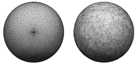
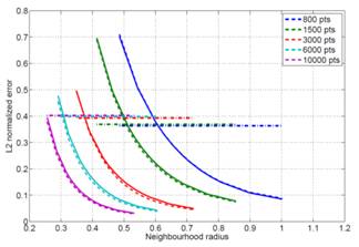
Additionally,
to test the influence of the triangulation on the operators, we repeated the
experiment with non-uniform sampling, as follows: ·
Points
were uniformly sampled on latitude-longitude coordinates, generating a much
denser sampling on the poles than on the Equator (Fig. 6, left). Results are
displayed in Fig. 7, left. We can see that the error of the cotangent
operator is now similar to the one of the diffusion operator. The use of Voronoi areas produces the best results in all cases. ·
Points
were randomly sampled on the surface of the sphere, generating a very uneven
triangulation (Fig. 6, right). Results are displayed in Fig. 7, right. We can
see that now the cotangent operator is worse than the diffusion-based
approach but there is also an increase in the size of the neighborhood needed
for optimal performance. The use of Voronoi areas
has little impact in performance. In summary,
the results we have so far suggest that we should use the Voronoi-area
correction for the diffusion operator, as it can bring an advantage for some
cases (both in terms of accuracy and size of neighborhood).
|
||||||||||||||||||||||||||||||
|
Laplacian spectrum and facial symmetry |
||||||||||||||||||||||||||||||
|
We
investigated the behavior of the Laplacian spectrum for variable degrees of
asymmetry of the human face. To this end, we started by constructing a
perfectly symmetric facial template obtained by averaging of 100 facial scans
(both the original and left-right mirrored version). Averaging was possible
thanks to the use of Least Squares Conformal Maps (LSCM) to have homologous
representations of all input surfaces (details here). Having a
symmetric template as described above makes it easy to introduce artificial
distortions to the facial surface. As an example, we produced an enlargement
of the left side of the face by scaling the distance of all left-side points
to the symmetry axis (mid-sagittal plane) by a
given percentage. Fig. 8 shows the distortion resulting from such a scaling
by a 20% factor.
The
re-sampling in the 2D domain was designed to produce points that correspond
to anatomically symmetric pairs. Recall that, in general, the human face is
not strictly symmetric and, in anatomical terms, the hypothetical axis of
bilateral symmetry is not contained in a plane. However, most research in
facial symmetry relies on the simplification of taking the mid-sagittal plane as the plane of bilateral symmetry, which
is then used to measure the deviations of one side with respect to the other
[Claes 2011]. This is
related to the direct use of 3D coordinates for analysis, while the facial
surface can be considered a 2D manifold embedded in 3D. In contrast, the
spectrum of the Laplacian relates to the structure of the manifold itself and
can be used for analysis without considering reflection over the mid-sagittal plane. So far, however, computation of this
spectrum is dependent on the extent of facial region that is captured, which
is extremely variable. Hence, the need and utility of the mesh normalization
that we perform based on LSCM. The spectrum
was computed by performing eigen-decomposition of
the Laplacian operator of each of the two templates mentioned above. The
results in this report correspond to the cotangent-based Laplacian (partial
inspection of the results with the diffusion-based Laplacian suggests that
results are not too different). An important
problem to compute the spectrum is that the, given a discrete Laplacian
operator L, we cannot guarantee that its eigenvectors u will be
real (i.e. in the general case they are complex). This happens because L is
not strictly symmetric, as it should be if it were a faithful representation
of its continuous equivalent. There are two main solutions to this problem [Zhang 2010]: i) force the operator to be symmetric, for example
by using = (L+LT)/2;
ii) decompose the Laplacian into a symmetric matrix S and a
mass matrix B, which simplifies obtaining real eigenvectors,
especially if B is diagonal. Evidently, the second solution is more
principled. The idea is to express the Laplacian as:
Both the
cotangent and diffusion approaches allow to easily separate L into a
symmetric matrix S and a diagonal matrix B-1. Doing some algebra it is
possible to show that an eigen-decomposition of L
can be obtained from the eigendecomposition of B-1/2SB-1/2. Specifically, the eigenvalues of B-1/2SB-1/2
are also eigenvalues of L and an
eigenvector v of B-1/2SB-1/2 can be transformed into
an eigenvector u of L by:
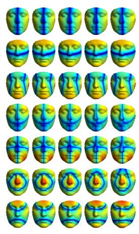
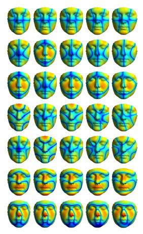
Fig. 9 show
the first 14 non-zero eigenvectors for the symmetric template and three
manipulated versions of it with increasing degree of asymmetry. To highlight
the patterns resulting from the eigenvectors, we have not plotted the values
of the eigenvectors v themselves, but a non-linear scaled version |u|1/4, where the exponential is
applied element-wise. The effect of this scaling is twofold: i) if highlights the zero-crossings (the dark-blue
lines); ii) it simplifies the perception of symmetry by converting
anti-symmetric values to symmetric ones. There are two
main observations: i) progressively adding
asymmetry resulted in also in a progressive modification of the spectral
components; ii) there were some shifts in the positions of certain
components, e.g. 9 with 10 and 11 with 12 in Fig. 3, presumably due to very
close eigenvalues, as discussed in the work by Ovsjanikov et al [Ovsjanikov 2008]. The above is
encouraging regarding the potential to measure symmetry in the spectral
domain, but it has to be put in context of the related work, especially since
before applying the spectral decomposition we have to put the surfaces in
dense correspondence. To the best of our knowledge, most efforts so far have
focused on the detection of the plane of bilateral symmetry or on the
alignment of a given shape with the mirrored (reflected) version of itself,
which is an over-simplification of the problem. We believe that this
spectral-based approach could help achieving a more principled analysis.
|
||||||||||||||||||||||||||||||
|
References |
||||||||||||||||||||||||||||||
|
[Atmosukarto 2010] I.
Atmosukarto, K. Wilamowska,
C. Heike and L.G. Shapiro. 3D
object classification using salient point patterns with application to
craniofacial research. Pattern Recognition, 43(1):1502–1517, 2010. [Belkin 2008] M. Bekin, J. Sun and Y. Wang. Discrete Laplace operator on
mesh surfaces. Proc. ACM Symp, on
computational geometry, pp 278-287, 2008 [Bronstein 2011] M.M. Bronstein and A.M. Bronstein. Shape
recognition with spectral distances. IEEE Transactions on Pattern
Analysis and Machine Intelligence, 33(5):1065–1071, 2011. [Claes 2011] P. Claes,
M. Walters, D. Vandermeulen and J.G. Clemen. Spatially-dense
3D facial asymmetry assessment in both typical and disordered growth.
Journal of Anatomy, 219(4):444–455, 2011. [Hormann 2007] K. Hormann, B. Levy and A. Sheffer.
Mesh
Parameterization: Theory and Practice. ACM SIGGRAPH course notes,
2007. [Hammond 2008] P. Hammond,
C Forster-Gibson, A.E. Chudley, et al. Face–brain
asymmetry in autism spectrum disorders. Molecular Psychiatry, 13,
614–623, 2008. [Khairy 2008] K. Khairy and J. Howard, Spherical
harmonics-based parametric deconvolution of 3-D
surface images using bending energy minimization. Medical Image
Analysis, 12(2): 217–227, 2008. [Levy 2006] B. Lévy. Laplace-Beltrami eigenfunctions.
Towards and algorithm that ‘understands’ geometry. Proc IEEE Conf
Shape Modeling and Applications, 2006. [Li 2006] H. Li and R. Hartley. New 3D Fourier
descriptors for genus-zero mesh objects. In Proc. Asian Conference on
Computer Vision. LNCS vol. 3851, pp 734–743, 2006. [Meyer 2002] M. Meyer, M. Desbrun,
P. Schröder and A.H. Barr. Discrete
differential-geometry operators for triangulated 2-manifolds. Proc
Visualization and Mathematics III, pp. 35–57, 2002. [Ovsjanikov 2008] M. Ovsjanikov, J. Sun,
and L. Guibas. Global
intrinsic symmetries of shapes. Computer Graphics Forum,
27(5):1341–1348, 2008. [Qiu 2008] A. Qiu, L. Younes and M.I. Miller.
Intrinsic
and extrinsic analysis in computational anatomy. Neuroimage,
39(4):1803–1814, 2008. [Reuter 2006] M. Reuter, F.E. Wolter
and N. Peinecke. Laplace-Beltrami spectra as ‘Shape DNA’ of surfaces and solids.
Computer Aided Design, 38(4):342-366, 2006. [Reuter 2009] M. Reuter, S. Biasotti,
D. Giorgi, et al. Discrete
Laplace-Beltrami Operators for Shape Analysis and
Segmentation. Computers & Graphics, 33(3): 381-390, 2009. [Ruggeri 2010] M.R. Ruggeri, G. Patane,
M. Spagnuolo and D. Saupe.
Spectral-driven
isometry-invariant matching of 3D shapes.
International Journal of Computer Vision, 89(2-3):248–265, 2010. [Taubin 1995] G. Taubin. A
signal processing approach to fair surface design. Proc SIGGRAPH, pp.
351-358, 1995. [Vallet 2008] B. Vallet. Function
bases on manifolds. PhD Thesis, Institut
National Polytechnique de Lorraine, France, 2008. [Wang 2007] S. Wang, Y. Wang, M. Jin et al. Conformal
Geometry and Its Applications on 3D Shape Matching, Recognition, and
Stitching. IEEE Transactions on Pattern Analysis and Machine
Intelligence, 29(7):1–12, 2007. [Zhang 2010] H. Zhang, O. van Kaick
and R. Dyer. Spectral
mesh processing. Computer Graphics Forum, 29(6):1865–1894, 2010. |
||||||||||||||||||||||||||||||
|
|
||||||||||||||||||||||||||||||
|
|
|
|
|
|||||||||||||||||||||||||||